Introduction to Landmark Models and the R package Landmarking

What is the landmark model used for?

Landmark models are used to dynamically predict the risk of an event for an individual. This means that an individual has a personalised risk prediction which is updated as new information is collected about them. Landmark models are particularly applicable in a medical setting where electronic health records (EHRs), such as GP records, are continually being updated with new data.

What is the landmark model?

The key idea behind landmark models is the concept of predefined landmark times. A landmark time is a time point (i.e. “landmark”) that we wish to make a risk prediction at. A model is built at the landmark time and this model is developed only using the data of individuals at risk (i.e. not censored or having experienced an event) at the landmark time.

For example, suppose that we want to predict the 5 year risk of a cardiovascular disease (CVD) event for a 45 year old patient. Then we would create a model for landmark time 45 years old using all the individuals that are in the risk set at 45 years old, and use this model to predict the risk of an event occurring for our new individual.

As we want to predict the risk of an event for an individual at a selection of time points, we define multiple landmark times and develop a model for each of these.

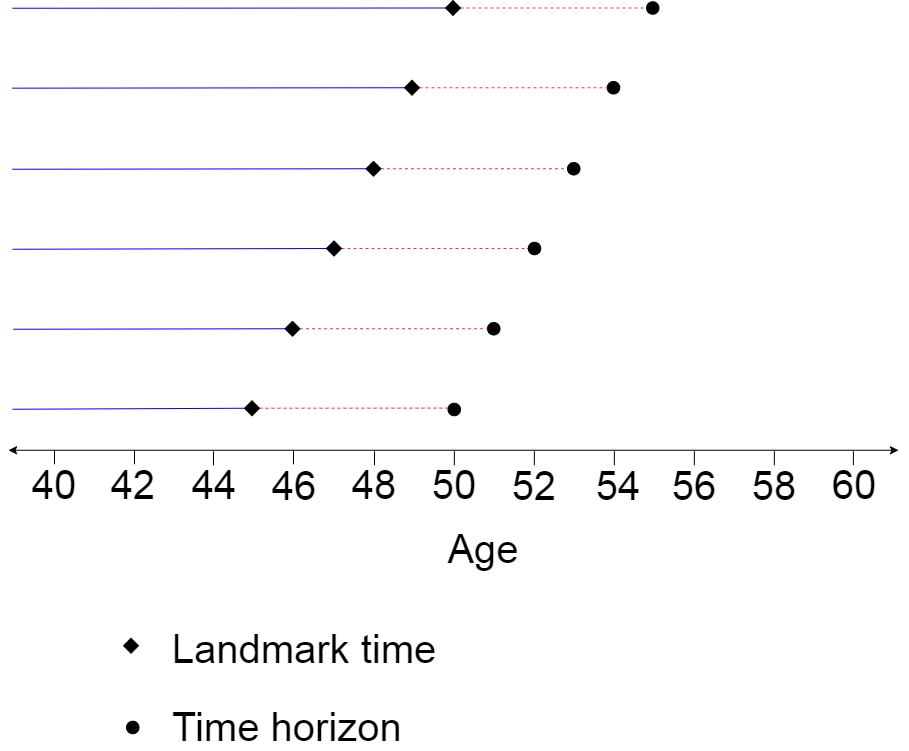
Continuing the example and supposing we wish to be able to predict the risk of CVD disease for any age between 45 and 50 years old, we define six landmark ages (45, … , 50 years old) and fit six models for each of these. This is demonstrated in Figure 1.

Figure 1: Illustration of a landmark model with six landmark times (ages 45 to 50 years). The blue solid line represents the time interval of longitudinal (repeat measures) data that feeds into the first stage of the two-stage landmark model. The red dashed line represents the time interval of the time-to-event data to be inputted into the survival model which is the second stage of the landmark model. Events after the time horizon need to be censored within this framework.

To form a model at each landmark age, landmark models use a two-stage model that is comprised of a extracting information from the longitudinal data which then feeds into survival model. The typical form of this is the last observation carried forward (LOCF) method and the Cox proportional hazards model respectively, although there are extensions and these are discussed in the `Features of the R package Landmarking’ section. Figure 1 shows the time intervals of the longitudinal (repeat measures) data and time-to-event data that is included when using the model, which is relative to the landmark age and time horizon. It should be noted that all the longitudinal (repeat measures) data may be used, including those passed the landmark age, in the first stage to develop a model. The survival model is fit only for the time-to-event data between the landmark age and the time horizon with all individuals censored at the time horizon. For a Cox proportional hazard survival model, this has the advantage that proportional hazards is only assumed for the short period between the landmark time and the time horizon rather than the entire period up until the end of study.

What are the advantages of the landmark model?

The other main statistical framework for this dynamic prediction problem is joint modelling. In comparison to joint modelling, the landmarking model is less computationally intensive and makes a less strong assumption about proportional hazards. Specifically this assumption only applies to the period between the landmark time and time horizon when using the landmark model.

Features of the R package Landmarking

The package Landmarking offers benefits over existing packages dynpred and landpred for landmark model analysis. In particular, three features of the package are outlined below.

1. Linear mixed effects modelling

The LME model is an alternative to using the LOCF method for the longitudinal data. LME modelling means that the entire history of a risk factor is used to evaluate predicted risk, as opposed to the LOCF model where only one (the most recent) measurement is used. Moreover the LME allows a patient to have missing values for the variables in the response.

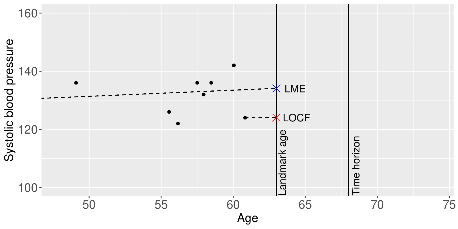
Figure 2 illustrates the use of these two types of models to predict systolic blood pressure at the landmark time. The LOCF model simply uses the most recently observed value of a risk factor. On the other hand, the LME model uses the entire history of the values of the risk factor from the individual, in combination with the trend in the risk factor from individuals used to develop the model. Using the Landmarking package, it is possible include a covariance structure in the random effects meaning that other risk factors can inform predictions. This improves the accuracy of the estimated value of the risk factor at the landmark time value compared to the LOCF model.

Figure 2: Comparison of the LOCF and LME model to predict systolic blood pressure at a landmark age for an individual with 8 repeat measures.

2. Competing risks modelling

The Landmarking R package has the ability to fit competing risks models for the survival model. There are two types of competing risks model that can be fit using this package, the Fine Gray model and the cause-specific model, using the parameter survival_submodel in the function fit_LOCF_landmark or fit_LME_landmark. The cause-specific model involves regression on the cause-specific hazard function. A covariate with a hazard rate greater than 1 is associated with an increased rate of the event of interest and less than 1 with a decreased rate of the event. Conversely, the Fine Gray model involves regression on the cumulative incidence function (CIF). In this case, a covariate with a hazard rate greater than 1 is associated with an increased incidence of the event of interest and less than 1 with a decreased incidence of the event. Their differences has led to the proposal that the cause-specific model is preferred when the aim is to study the aetiology of a disease, and the Fine Gray model is preferred when the aim is prediction of the risk of an event.

3. Cross-validation

Another feature of this package is that is makes it easy to perform k-fold cross validation. The function add_cv_number assigns a fold to each individual in a dataset. When multiple landmark ages are defined within functions fit_LOCF_landmark or fit_LME_landmark, the cross validation folds are kept consistent for individuals across the corresponding landmark models.

How is the landmark model fit within the R package Landmarking?

The functions fit_LOCF_landmark and fit_LME_landmark are used to fit the landmark model in this package. See the vignette How to use the R package ‘Landmarking’ to see a worked example which uses these functions.

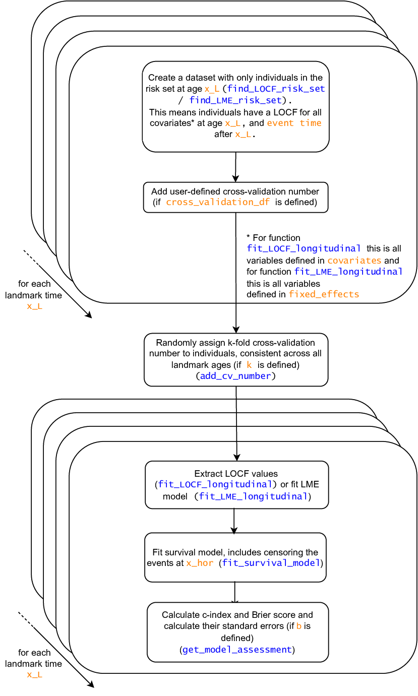
Here is a diagram that represents the functions fit_LOCF_landmark (selecting option fit_LOCF_longitudinal) and fit_LME_landmark (selecting option fit_LME_longitudinal) to show how they are made up of their helper functions. All these functions are available with the R package Landmarking.

The first step of the functions fit_LOCF_landmark and fit_LME_landmark is forming the datasets that correspond to each value of the landmark ages in x_L. These datasets will contain only the data of the individuals in the risk set at each landmark age x_L. To be in the risk set at age x_L the individual must have:

• entered the study at a time up to and including the landmark age x_L. This means that the individual has at least one LOCF value for all variables in covariate for the case of fit_LOCF_landmark, or at least one LOCF value for all variables in predictors_LME for the case of fit_LME_landmark. This condition is necessary for the LOCF approach as the LOCF values at the landmark age x_L are extracted for all covariates and so at least one observation is needed of each of these. This condition is necessary for the LME approach, as the LOCF values at the landmark age x_L are extracted for predictors_LME and so at least one observation is needed of each of these. On the other hand, the function fit_LME_landmark allows for missing observations in responses_LME by the landmark age.

• exited the study after and not including time x_L.

This is performed using the functions find_LOCF_risk_set or find_LME_risk_set.

After this dataset is formed for each of the landmark ages, the second step involves adding the cross-validation fold to the individuals in the dataset. The datasets that were just formed are re-combined in order to ensure that the cross-validation fold assignment is consistent across each of the datasets. In other words the individual that is in the risk set at one landmark time has the same cross-validation number as when they are in the risk set at another landmark time. The cross-validation folds may be defined in two ways:

• the user sets parameter k which randomly assigns cross-validation folds to each individual using the function add_cv_number

• the user sets parameter cross_validation_df which refers to a data frame that contains the user-defined assignment of cross-validation folds.

Alternatively, no cross-validation is performed.

In the third and fourth steps the landmark model is fitted separately to each of the datasets that correspond to a landmark age x_L (with the cross_validation_number added). If the parameters k or cross_validation_df are used, then the landmark model is formed using the training dataset and applied to the test dataset.

In the third step, function fit_LOCF_longitudinal or fit_LME_longitudinal is used. The function fit_LOCF_longitudinal extracts the LOCF value for each of the covariates in data_long up to (and including) time x_L. On the other hand, the function fit_LME_longitudinal fits a multivariate linear mixed effects model (with unstructured covariance) to the training dataset. The model contains a random intercept and random slope (if random_slope_longitudinal=TRUE). Once this model is fitted, the BLUP estimates of the response variables (and slopes if random_slope_survival=TRUE is used) are calculated for the test dataset. These values, along with the LOCF value for each of the covariates in predictors_LME, are used as the covariates in the survival model. For more information see help(fit_LME_longitudinal).

Fitting the survival model is performed using fit_survival_model. This function censors the individuals at the horizon time x_hor and then fits the survival submodel specified in the function arguments. There are three choices for this model (standard Cox model, Fine Gray model, and cause-specific model). For more information see help(fit_survival_model).

In the fifth step, the performance of the model is assessed using c-index and Brier score. If the parameter b is defined, then the bootstrap estimates of the c-index and Brier score are calculated as well. For both the c-index and Brier score calculations, inverse probability censoring weighting (IPCW) is used to create weights which account for the occurrence of censoring. The censoring model assumes for this function is the Kaplan Meier model, i.e. censoring occurs independently of covariates.